Creating ACT-like genomic comparison images : a dummies guide for biologists
In this blog I am going to describe the steps you can take to install R, genoPlotR, a few plugins in a linux machine (I have Ubuntu 16 which I upgraded in my biolinux 8 operating system) and other software and make a publication quality ACT-like image of a comparison of genomic DNA sequences or genomic regions.
1) Installing or upgrading R
My machine had R-3.2.3. This may be good enough but if you’re going to start installing things and creating files you want your work to give you “rewards” in the form of a platform you can use for as long as possible before you start finding that the new packages you want to use are incompatible with your old R version and you start having to search in archives for compatible packages and help. There are various help pages on the web on how to migrate your work if you do need to move from an older version of R to a newer one, I’m not going to go into that here but you can find most of the information you need here:
https://cran.r-project.org/doc/manuals/R-admin.html#Getting-and-unpacking-the-sources
The guide directs you to https://CRAN.R-project.org/mirrors.html to obtain R. This link gives you a list of mirrors from which you have to chose one. In my case I chose the first UK link what is for the University of Bristol. If you select that mirror you get some information on R such as the latest release (Monday 2016-10-31, Sincere Pumpkin Patch) R-3.3.2.tar.gz) and options to download R for Linux, Mac, or Windows. Once you click on the option to download you then need to select your linux version from the next page (I picked ubuntu).
The lazy way in which you can then install R is using typing the following text into a terminal:
sudo apt-get install r-base r-base-dev
In my case I got the following messages:
r-base is already the newest version (3.2.3-4).
r-base-dev is already the newest version (3.2.3-4).
Be aware that because of how rapidly things change and how databases and links are not always updated or maintained you have to expect that you are being lied to and double-check everything.
If you have an eye for detail and followed the guide above you’ll be blinking at the 3.2.3 and wondering how that is the new version when you’ve just been told the new version is 3.3.2.
Unfortunately that’s life. Ignore the message and download the newest version of R . There’s a link to “R Sources” in the left sidebar under Software which gives you a link to R-3.3.2.tar.gz.
Download the file to a folder of your choice and unpack it with
tar -xf R-3.3.2.tar.gz
The R manual gives a list of ways to install the new R version on your system.
I just used
./configure
Make
You should get a list of messages on the lines of:
R is now configured for x86_64-pc-linux-gnu
Source directory: .
Installation directory: /usr/local
… etc.
Congratulations, you now have a up-to-date version or R.
In my case I already had R-3.2.3 and because its not very big, just in case I happen to need to use a package which is incompatible with newer versions I decided to keep it. In order to have the newer version open when I type R in my command line I renamed R in the folder /usr/bin to R-3.2.3 and copied my new R file to /usr/local/bin
R 3.3.2 now opens by simply typing R in a terminal from any folder location.
2) Installing some R packages
To use R as a tool to aid in the analysis of biological data you probably don’t want to have to write your own scripts. The next thing to do if this is the case is install packages which will do the jobs you need to do for you.
GenoPlotR
A nice and easy to use package for creating genomic or cluster comparison files is genoPlotR, made and maintained by Lionel Guy and I’m going to continue talking about the 0.8.4 version (2015-07-02).
I chose this for several reasons. One is that it includes very convenient methods for importing your data from genbank files, blast files and even alignment files. This issue is not trivial because if your data is in various formats of gff, gff3, gtf annotation files and the tools you want to use tell you that you have to supply files with three columns with specific information then you either have to rewrite the information you need based on the annotation files you have or spend a few days tidying them up with various scripts. Also in my case I am a fan of ACT (Sanger) and find the similarity in its images and the convenience of using the same files to manipulate and annotate your files in ACT and Artemis then feed the same files into genoPlotR very useful.
To install packages start up R in your working folder by typing:
R
From there if you have a newly installed R equip yourself with Bioconductor:
source(“https://bioconductor.org/biocLite.R”)
biocLite()
If you’re new to R check out http://bioconductor.org/packages/release/BiocViews.html#___Software to get an idea as to what other packages you can use from bioconductor.
Next install the genoPlotR, its dependencies and any of the other packages you may need.
biocLite(c(“ade4″,”genbankr”,“ggbio”))
install.packages(“genoPlotR”)
You can exit R by typing q()
3) Using R from command line
Now you have everything installed you need to start creating your R analysis pipeline.
You can just write commands in your terminal but I’m going to recommend creating a file in “getedit” or “notepad++” with your pipeline. I’m going to call mine “R_cluster_graphics.analysis”
You can add comments of what you are doing by beginning lines with #.
At any point you can run the script to see what comes out with the command:
R CMD BATCH R_cluster_graphics.analysis
This will create file named R_cluster_graphics.analysis.Rout in the folder you ran it from which you can open and check for error messages and for messages which answer questions in your analysis pipeline for example is.dna_seg which returns TRUE or FALSE.
First add commands to load the packages you need to use:
##Libraries
library(ggbio)
library(genoPlotR)
library(ade4)
library(grid)
## State where you would like your images to be save to:
imgPath <- “../img”
pdfPath <- “../pdfs”
imgPath <- “/media/…/genoPlotR”
pdfPath <- “/media/…/genoPlotR”
##Import your genbank data (referred to as dna_seg):
SampleA
SampleB
#check dna_seq identity
is.dna_seg(SampleA)
is.dna_seg(SampleB)
#Create your Comparison files.
You can make these with blastall or blast+ in a terminal by formatting one sequence as a database and running a blastn or tblastx using the first dna_seg as input and the second one as the database. Here is an example of how to do this for two fasta files that match your genbank files and are in the same folder:
1) Navigate to your folder.
2) Format your database with:
formatdb -i SampleB.fasta -p F
3) Run a blastall search:
blastall -p tblastx -d /media/…/ SampleB.fasta -i /media/…/ SampleA.fasta -o SampleA_SampleB.tblastx -m 9
Alternatively you can also use the NCBI online blast tool at https://blast.ncbi.nlm.nih.gov/Blast.cgi?PROGRAM=blastn&PAGE_TYPE=BlastSearch&LINK_LOC=blasthome and download your comparison files from there.
#Import your Comparison files.
SampleA_SampleB.comparison <- read_comparison_from_blast(“/media/…/SampleA_SampleB.tblastx”, sort_by = “per_id”,filt_high_evalue = NULL,filt_low_per_id =NULL,filt_length = NULL,color_scheme = NULL)
etc.
#check that your comparison file is acceptable:
is.comparison(SampleA_SampleB.comparison)
If you would like to have a distance tree in your image make an alignment and a corresponding dendrogram. There are a number of command line tools and GUI software packages which can do this.
In my case I used MEGA7 to make an alignment with the muscle algorithm, you can try other algorithms and especially if your sequences are large or dissimilar I would recommend trying a few algorithms and picking the most appropriate alignment. You can get various version of MEGA from http://megasoftware.net/ I used the command line version of MEGA7 by opening megaproto (go to the installation folder and type megaproto), selected “non coding nucleotide alignment” and “muscle nuc alignment” from the Align option in the toolbar and changed the cluster method to Neighbor Joining for all iterations then saved these settings as a .mao file.
To make life easier I joined all my fasta sequences with the command
cat sequence1.fasta sequence2.fasta etc > allsequences.fasta
I then ran the alignment with the command:
/media/…/MEGA7/megacc -a /media/…/nucleotide_align.mao -d /media/…/allsequences.fasta -o MEGA7_allsequences.alignment
I then used the alignment to make a tree with RAxML version 8.2.4. which you can get from GitHub at https://github.com/stamatak/standard-RAxML
If you would are also going to use use RAxML check which version you need. If you are able to use multiple threads I would definitely pick the Pthreads option. Especially if you are planning on making trees out of huge alignments in the future I would definitely pick the best version you can. In my case I used the AVX version which is compatible with Intel i7.
You can download the files with the command
git clone https://github.com/stamatak/standard-RAxML.git
and install the appropriate version in the manner described in the Readme file in the software folder. In my case it was:
make -f Makefile.AVX.PTHREADS.gcc
rm *.o
Run RAxML to make your tree. I used the BS and ML recommended settings from the RAxML manual. It didn’t like my MEGA7 alignment so I converted it to a phylip alignment. There are many tools that can handle this but since I don’t have much on my new computer yet I used this link http://sequenceconversion.bugaco.com/converter/biology/sequences/
RAxMLHPC-PTHREADS-AVX -f a -x 12345 -p 12345 -# 100 -m GTRGAMMA -s /media/…/MEGA7_alignment.phylip -n MEGA7_alignment.RAxML -T 6
Note: If you can’t use threads remove the -T 6 bit
This creates a RAxML_bestTree.MEGA7_alignment.RAxML file
You can view your tree using various software packages. One example is dendroscope which comes with biolinux and by typing dendroscope into a terminal it opens a graphical user interphase (GUI) from which you can navigate to your tree file and quickly visualize it.
Give R your tree information by pasting the data from the RAxML_bestTree.MEGA7_alignment.RAxML file into a tree<- newick2phylog(“”) command :
tree<- newick2phylog(“((SampleA:0.10250953446912315636,SampleB:0.09775744461960976517):0.01209692024574308099,((SampleC:0.04104447134815911863,SampleD:0.06305211466588933611):0.01132124623294956944,SampleE:0.11080167962495350575):0.01743359660415144674,SampleF:0.10269874269575925141):0.0;”)
#Pick the shapes you would like your CDS to appear as. I used arrows. You can see the other options with the command: gene_types()
gene_types(auto = FALSE)
SampleA$gene_type <- “arrows”
SampleB$gene_type <- “arrows”
etc
#Give you dna_seg sequences CDS annotation
annotA <-auto_annotate(SampleA)
annotR <-auto_annotate(SampleB)
etc
# Make your DNA-comparison image
pdf(file.path(pdfPath, “My_SampleABetc_comparison.pdf”), h=7, w=10)
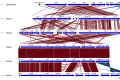
plot_gene_map(dna_segs=list(SampleA, SampleB, next samples), comparisons=list(SampleA_SampleB.comparison, next comparisons),annotations=list(annotA,annotB,next annotations),override_color_schemes=TRUE, global_color_scheme=c(“e_value”, “auto”, “red_blue”, “0.5”),dna_seg_labels=c(“SampleA”,”SampleB”,”next labels”),tree=tree)
This should give you a nice comparison pdf which looks like what you always wanted ACT images to look like, in the folder you specified for pdfPath above.
The manual gives lots of detailed information on how you can change the parameters above to alter your image size, colours, annotation etc but I would like to mention that the power of using a file with the commands above to make your image is that once you have it and see what the output looks like you can go back to your genbank files and add any new CDS you discover or change their names then run the script again with “R CMD BATCH R_cluster_graphics.analysis” to get the new image. You can also make several different trees, call them tree1, tree2, tree3 then make several comparison images just by rerunning the script once with more copies of the “# Make your DNA-comparison image” commands with the appropriate tree name specified and the other lists and labels in the correct order. Here is an example:
## Make your comparison tree1
pdf(file.path(pdfPath, “My_SampleABetc_tree1.pdf”), h=7, w=10)
plot_gene_map(dna_segs=list(SampleA, SampleB, next samples), comparisons=list(SampleA_SampleB.comparison, next comparisons),annotations=list(annotA,annotB,next annotations),override_color_schemes=TRUE, global_color_scheme=c(“e_value”, “auto”, “red_blue”, “0.5”),dna_seg_labels=c(“SampleA”,”SampleB”,”next labels”),tree=tree1)
## Make comparison image for tree2 (you may need to make and specify more blastall comparison files)
pdf(file.path(pdfPath, “My_SampleABetc_tree2.pdf”), h=7, w=10)
plot_gene_map(dna_segs=list(SampleB, SampleA, next samples), comparisons=list(SampleB_SampleA.comparison, next comparisons),annotations=list(annotB,annotA,next annotations),override_color_schemes=TRUE, global_color_scheme=c(“e_value”, “auto”, “red_blue”, “0.5”),dna_seg_labels=c(“SampleB”,”SampleA”,”next labels”),tree=tree2)
#You can also add different types of annotation and gene_types by giving them different names then making even more images each with a different type of annotation or graphics for your CDS.
4) Check your images
Hopefully if you followed this guide you should have some very pretty pdf files of your genomic DNA comparisons now. It is a good idea to scrutinize your images and make sure they look realistic. If it looks like the comparison lines don’t seem quite right between two or more samples, for example you have 3 conserved geneA sets but the comparison lines give good identity to irrelevant regions, check that you used the correct reference and input sequences in your blast and try supplying a comparison file with the sequences give in the reverse order. Unfortunately genoPlotR does not automatically get the sample information from the blast files so this is something you have to be careful about.
For examples of the output images please see the genoPlotR page and a publication with an image made with genoPlotR.
5) Final words
I would like to give thanks to Lionel Guy himself in this post as besides creating this very useful and easy-to-use R tool (compared to many other R tools) in two instances where I could not tell from the manual how to deal with my annotations and tree, he responded in less than 24 hours to my e-mailed questions with precise and very helpful answers. This blog is by no means a substitute for the software manuals or a claim of expertise but rather what I hope is a simple guide for biologists which are unfamiliar with software manuals, R code and the sort of mistakes they can make if you are not aware of issues such as order of commands and recognition of data structures and need a simple guide on how to go about starting to use R to get a publication-quality image that looks like your lovely ACT comparison.
Reading material:
- ACT:Carver, Tim J., et al. “ACT: the Artemis comparison tool.” Bioinformatics 21.16 (2005): 3422-3423 http://www.sanger.ac.uk/science/tools/artemis-comparison-tool-act
- Artemis: Rutherford, Kim, et al. “Artemis: sequence visualization and annotation.” Bioinformatics 16.10 (2000): 944-945http://www.sanger.ac.uk/science/tools/artemis
- genoPlotR: Guy, Lionel, Jens Roat Kultima, and Siv GE Andersson. “genoPlotR: comparative gene and genome visualization in R.” Bioinformatics 26.18 (2010): 2334-2335 https://cran.r-project.org/web/packages/genoPlotR/index.html
- BLAST: http://www.ncbi.nlm.nih.gov/blast
- Bioconductor: http://bioconductor.org/
- MEGA7: http://megasoftware.net/
- RAxML: A. Stamatakis: “RAxML Version 8: A tool for Phylogenetic Analysis and Post-Analysis of Large Phylogenies”. In Bioinformatics, 2014, open access.
- GitHub: https://github.com/
- Biolinux: http://environmentalomics.org/bio-linux/
- Hatziioanou D., Gherghisan-Filip C., Saalbach G., Horn N., Wegmann U., Duncan S., Flint H, Mayer M.J., Narbad A. Discovery of a novel lantibiotic nisin O from Blautia obeum A2-162, isolated from the human gastrointestinal tract, Microbiology (2017) 163: 1292-1305 (genoPlotR image made using this process).


2017 Biology week lectures: Vaccine research overview from key virologists
Prologue
Having recently moved back to the UK I was not aware that there is such a thing as a biology week. Thankfully the Royal Society of Biology made sure to bring this celebration to my immediate attention by broadcasting it on its web-page so that I became aware of both its existence and some of the lectures and events on during this celebration of biology.
Scrolling down the list of events from the Royal Society of Biology webpage I identified two promising talks about vaccines and promptly booked myself a place in them. This blog is dedicated to sharing some of the insights from these lectures:
- “Around the world in 80 days” by Professor Wendy Barclay, Chair in Influenza virology at Imperial College London which would be hosted as part of the RSB AGM in Reading
- “Vaccines for a 21st century society” by Professor Rino Rappuoli, Chief Scientist & Head of External R&D at GSK Vaccines as part of the Environmental Microbiology Annual Lecture 2017 hosted by the sfam in London
Part 1: Professor Wendy Barclay -Influenza A virus overview
Wendy gave a lovely talk starting with a brief description of influenza virus components and with the importance and impact of influenza in society which included a description of yearly spikes of occurrence, epidemiological and pandemic occurrences and Prince Philip’s statement that he had “not had flu for 40 years”. She also mentioned the potential reasons for this such as:


Wendy then went on to talk about the barriers viruses face when attempting to infect a different host type.
Influenza species are categorised as A (avian), B (human) and C. The natural hosts of influenza A virus are birds where typical infections with influenza A virus do not show any symptoms. Some strains however cause systemic infection with involvement of the central nervous system.
In wild ducks, influenza viruses replicate preferentially in the cells lining the intestinal tract, cause no disease signs, and are excreted in high concentrations in the faeces (Webster 1992 & 1978).
She pointed out while showing us a number of images of birds such as pigeons, ducks, swans and chickens in close proximity to humans how infrequently humans become infected with avian influenza despite our frequent exposure to the avian virus infested birds. Although, she mentioned, lethality is high in the known cases that humans have caught avian influenza the avian virus is usually incapable of becoming airborne and transmitted to further humans from a human host meaning that the zoonotic strain normally does not spread from the infected human. Indeed according to Wan et al approximately 60% of 385 human infections with avian Influenza in Vietnam have been fatal [3], but very few have been transmitted from person to person [4]. Infections are usually acquired by contact with H5N1 infected poultry or poultry products, and the H5N1 viruses isolated from human cases are often virtually identical to isolates from poultry [5].
She went on to explain that viruses have adapted over the centuries to infect specific hosts in a way which permits viral infection and replication in a manner which is less detrimental to their favourite host. This evolution includes adaption to have a preference for certain mammalian cell receptors, for the virions to be stable under different pH conditions, to be able to make use of the their viral RNA-dependent RNA polymerase in its host cells.
In order to understand these preferences we need to understand a bit about the nature of influenza virus structure and biology.
The influenza A virus comprises of an outer host derived lipid bilayer embedded with the virus-encoded glycoproteins hemagglutinin (HA) and neuraminidase (NA) and matrix protein 2 (M2), and within that an inner shell of matrix protein which protects the nucleocapsids of the viral genome at the centre of the virus particles. The lipid bilayer of Influenza B contains an addition NB component and Influenza C contains only an M2 protein and the hemagglutinin–exterase-fusion (HEF) protein that combines the functions of HA and NA.
HA mediates the viral binding to host cell receptors. Human influenza preferentially binds α2,6-linked sialyloligosaccharide receptors (mostly found in the upper respiratory tract) and avian influenza prefers α2,3-linked sialyloligosaccharide receptors which are more abundant in the lower respiratory tract. The M2 ion channel equilibrates the pH across the viral membrane and NA cleaves sialyloligosaccharide residues (oligosaccharides with one or more sialic acid residues) from host cell surfaces aiding in the release of the viral particles.
The influenza virus genome comprises of eight single-stranded, negative-sense RNA molecules (vRNA) as well as multiple copies of NP (Nucleoprotein) with which it forms a viral ribonucleoprotein (vRNP) complex with a single RNA polymerase which is a trimer or the three proteins; PA (Polymerase acidic protein), PB1 (RNA-directed RNA polymerase catalytic subunit)and PB2 (Polymerase basic protein 2).
Hundreds of mammalian cellular factors have been identified that affect virus replication or whose expression is modulated by the virus (Zhao M. 2017). As can be expected a large number of those interacting proteins interact with the viral polymerase.
A number of studies have found that the avian viral RNA polymerase functions weakly in human cells while certain mutations, particularly of its PB2 protein, are selected during adaption of the avian strains to mammalian cells (Mänz B 2013, Subbarao, E. 1993, Naffakh, N. 2008). Particularly residue 627 of PB2 which sports a lysine (rarely an arginine) in human Influenza and a glutamic acid in avian Influenza has been found to play a crucial role to host adaption.
- The single amino acid substitution, from glutamic acid to lysine at position 627 of the PB2 protein, converts a nonlethal H5N1 influenza A virus isolated from a human to a lethal virus in mice (Shinya).
- In one study the acquisition of an avian PB2 in an otherwise human Influenza restricted the viruses replication in mammalian cells (Clements). After several passages through mammalian cells the viral chimera acquired the ability to replicate by acquisition of the PB2 E627K mutation (Subbarao).
- The 1918 pandemic strain had a lysine residue at position 627 although the PB2 gene was otherwise avian virus-like implying that it did not acquire host adaption by re-assortment (Taubenberger et al). A total of ten amino acid changes in the polymerase proteins consistently differentiate the 1918 and subsequent human influenza virus sequences from avian virus sequences, five of which were to the PB2 protein. Out of 253 available PB2 sequences from human H1N1, H2N2 and H3N2 isolates, these five changes are almost completely preserved, with the exception that two recent H3N2 isolates have the avian Lys residue at position 702. Only a small number of avian influenza isolates show any of these five changes, and it is intriguing that almost all of these isolates are from HPAI H5N1 or H7N7 viruses, or from the H9N2 lineage that infected a small number of humans in China in the late 1990s (ref. 29). Notably, a number of the same changes have been found in recently circulating, highly pathogenic H5N1 viruses that have caused illness and death in humans and are feared to be the precursors of a new influenza pandemic.
- In highly pathogenic avian influenza (HPAI) H5N1 which arose in Vietnam in 2004 and 2005 lysine 627 and asparagine 701 were both correlated with fatal disease in infected patients (de Jong )
- It is interesting that in avian cells virus polymerases containing PB2 627K are only two times more efficient than those with 627E
- E627K was present in the single fatal human infection during the HPAI H7N7 outbreak in the Netherlands in 2003 (Fouchier ). A highly pathogenic avian influenza A virus of subtype H7N7, closely related to low pathogenic virus isolates obtained from wild ducks, was isolated from chickens. The same virus was detected subsequently in 86 humans who handled affected poultry and in three of their family members. Of these 89 patients, 78 presented with conjunctivitis, 5 presented with conjunctivitis and influenza-like illness, 2 presented with influenza-like illness, and 4 did not fit the case definitions. Influenza-like illnesses were generally mild, but a fatal case of pneumonia in combination with acute respiratory distress syndrome occurred also.Most virus isolates obtained from humans, including probable secondary cases, had not accumulated significant mutations. However, the virus isolated from the fatal case displayed 14 amino acid substitutions, some of which may be associated with enhanced disease in this case.
- Six influenza isolates were obtained from four different provinces of Thailand during the avian influenza outbreak in Asia from late 2003 to May 2004 (Puthavathana et al).
- In Hong Kong in 1997 and 2003, highly pathogenic avian influenza (HPAI) of subtype H5N1 was transmitted from birds to humans, of whom at least seven died (8–13).
- Pandemics of 1918 (H1N1), 1957 (H2N2), and 1968 (H3N2) were caused by influenza viruses harboring HA and NA genes of avian or swine origin (1, 2).
In search of the mechanisms which control the Influenza restriction to different hosts Wendy’s team focused on the activity of influenza A viral polymerase in heterokaryons formed between avian (DF1) and human (293T) cells. In their work they found that there is no restriction factor for avian-derived polymerase present in human cells. Thus, the restriction in human cells is likely the consequence of the absence of an interaction or a low-affinity interaction with an essential cofactor. Finally, this work also gives an explanation for the natural selection of the adaptative mutation E627K in PB2 by implying the presence of a human-specific positive cell factor that enhances replication of polymerases only when the PB2 627K motif is present. (Moncorgé O. et al, 2010).
Following this discovery Wendy’s team went on to look for a potential interacting factor. They found that the mammalian protein ANP32A interacts with the viral RNA polymerase PB2 protein and that “species-specific difference in host protein ANP32A accounts for the sub-optimal function of avian virus polymerase in mammalian cells”.
Wendy showed us an alignment of ANP32A protein sequences from animal and bird species which made it obvious that this protein is highly conserved and that an insertion event added a 33 amino sequence to avian ANP32A . This insertion was not present in human, porcine or ostrich ANP32A. She went on to explain the hypothesis that avian influenza must have adapted to bird species after the evolutionary event which separated mammals and land bound birds such as Ostriches from birds of flight. She presented some of he teams work which showed that the short added sequence present in avian ANP32A made all the difference between the species that avian influenza could infect because it determined whether the avian virus polymerase was able to function or not permitting viral replication in the host cells.
Wendy went on to show some metrics on influenza vaccination. She showed some epidemiological data that suggested that occurrences reduced during school breaks making children the largest culprits of infection spikes.
She then introduced us to the concept of nasal vaccination of four attenuated influenza species in natural lipid particles delivered through a nasal spray which has adapted to survival at lower temperatures such as those found in the nose cavity of humans confining the viral infection anatomically by temperature restriction and eliminating the need for injections. Other major benefits of this type of vaccination include activation of both mucosal and systemic immune response, an increased safety profile as the vaccine is not injected and does not contain in potentially harmful adjuvants and broad specificity antibody responses which could protect against viral/bacterial strains not included in the vaccine. Most notably it was interesting to see that after vaccination reported infections were reduced not only on the year of vaccination but also the following year. She voiced concerns over the availability of this powerful vaccination strategy which protects against the strains found in UK as data from the US showed that one of the four influenza species which caused the majority of infections in US appears not to be as successful as the other three strains in protecting against infection when used in the nasal vaccine.
Finally she introduced pH lowering nasal sprays as an example of how pH influences influenza virus stability and its ability to infect cells. Influenza virus enters its host cells via endosomes/lysosomes and needed the acidic pH of these endosomes to release its DNA from the viral capsid into the host cell cytoplasm. Lowering of the nasal cavity pH with an acidic spray is therefore be a logical methodology for degrading the virus coat and exposing its genetic material to mucosal and environmental enzymes which can degrade it and protect from infection.
The lecture was followed by a questions and answers session. Intrigued by the fact that avian influenza which infects humans working in close proximity with birds do not usually transmit the virus to others and having in mind methods of horizontal DNA transfer and interesting findings of DNA both becoming encapsulated in viral particles and binding to them in viral DNA aggregates I took this opportunity to ask Wendy her opinion on the ability of influenza viruses to evolve not only by mutation but also by horizontal transfer of pieces of DNA from other species. Wendy stressed that picked up DNA would really have to confer the virus a selective advantage for it to be kept and integrated into its genome but to my delight she confirmed my suspicions by going on to mention that they have frequently found fragments of host DNA (ribosomal and other types) when sequencing viral genomes.
See also:
Further reading:
- Webster, Robert G., et al. “Evolution and ecology of influenza A viruses.” Microbiological reviews 56.1 (1992): 152-179 (inlcudes electron micrographs of Influenza A).
- Webster, Robert G., et al. “Intestinal influenza: replication and characterization of influenza viruses in ducks.” Virology 84.2 (1978): 268-278.
- Zhao, Mengmeng, Lingyan Wang, and Shitao Li. “Influenza A Virus–Host Protein Interactions Control Viral Pathogenesis.” International journal of molecular sciences 18.8 (2017): 1673.
- http://jvi.asm.org/content/65/1/232.short nuclear transport
- https://virologyj.biomedcentral.com/articles/10.1186/1743-422X-4-49 nuclear localization sequences
- Moncorgé O, Mura M, Barclay WS. Evidence for Avian and Human Host Cell Factors That Affect the Activity of Influenza Virus Polymerase . Journal of Virology. 2010;84(19):9978-9986. doi:10.1128/JVI.01134-10.
- Mänz, Benjamin, Martin Schwemmle, and Linda Brunotte. “Adaptation of avian influenza A virus polymerase in mammals to overcome the host species barrier.” Journal of virology87.13 (2013): 7200-7209.
- Subbarao, E. Kanta, and B. R. Murphy. “A single amino acid in the PB2 gene of influenza A virus is a determinant of host range.” Journal of virology 67.4 (1993): 1761-1764.
- Naffakh, Nadia, et al. “Host restriction of avian influenza viruses at the level of the ribonucleoproteins.” Annu. Rev. Microbiol. 62 (2008): 403-424.
- Hatta, Masato, et al. “Growth of H5N1 influenza A viruses in the upper respiratory tracts of mice.” PLoS pathogens 3.10 (2007): e133.
- Scull, Margaret A., et al. “Avian Influenza virus glycoproteins restrict virus replication and spread through human airway epithelium at temperatures of the proximal airways.” PLoS pathogens 5.5 (2009): e1000424
- Taubenberger, Jeffery K., et al. “Characterization of the 1918 influenza virus polymerase genes.” Nature 437.7060 (2005): 889-893.
- de Jong, Menno D., et al. “Fatal outcome of human influenza A (H5N1) is associated with high viral load and hypercytokinemia.” Nature medicine 12.10 (2006): 1203-1207.
- Wan, Xiu-Feng, et al. “Evolution of highly pathogenic H5N1 avian influenza viruses in Vietnam between 2001 and 2007.” PloS one 3.10 (2008): e3462.
- Fouchier, R. A. et al. Avian influenza A virus (H7N7) associated with human conjunctivitis and a fatal case of acute respiratory distress syndrome. Proc. Natl Acad. Sci. USA 101, 1356–1361 (2004)
- Shinya, K. et al. PB2 amino acid at position 627 affects replicative efficiency, but not cell tropism, of Hong Kong H5N1 influenza A viruses in mice. Virology 320, 258–266 (2004)
- Puthavathana, Pilaipan, et al. “Molecular characterization of the complete genome of human influenza H5N1 virus isolates from Thailand.” Journal of General Virology 86.2 (2005): 423-433.


New CRISPR-Cas9 screening method identifies “magic bullet” molecular targeted therapy candidates to help the body’s immune system fight cancer
Molecular targeted therapy (composed of small-molecule drugs and monoclonal antibodies) blocks the growth and spread of cancer by interfering with specific molecules that are critical for tumor progression such as checkpoint inhibitors1.
The potential of this approach was recognized in 1998, when the antibody trastuzumab (Herceptin) against receptor tyrosine kinase HER2 was approved by the FDA for treatment of patients with HER2-receptor positive metastatic breast cancer2. Subsequently in 2001, imatinib (Gleevec), a small molecule kinase inhibitor3 received FDA approval for the treatment of chronic myeloid leukemia (CML). Imatinib was the first rationally designed small-molecule inhibitor, it made the cover of “TIME” magazine as the “magic bullet” and was considered as the start of a new era in anticancer drug discovery4. In recent years our advances in tumor immunology and immunotherapy have led to FDA and EMA approval of several checkpoint inhibitors such as PD-1 and PD-L1 in clinical practice5.
Dr W. Nick Haining, an associate professor of paediatrics at Harvard Medical School, associate member of the Broad Institute of MIT and Harvard and team leader of the Dana-Farber/Boston Children’s team, in a recent press release voiced his concerns that despite the clinical success of PD-1 checkpoint inhibitors the majority of patients’ cancer does not respond to this treatment. This has triggered a number of studies looking at drugs to increase the number of patients responding to PD-1 inhibitor treatment.
In their recent publication6 Dr Hainings’ team showed that CRISPR-Cas9 targeted genome editing technology which up to now has been used to identifying genes required by tumor cells for proliferation, metastasis and drug resistance7,8, could be used to look at the interaction of tumor cells with the natural immune system to identify candidate drug targets for sensitizing cancerous cells to the immune system. They did this by disabling 2368 genes in a library of melanoma cells and transplanting the cells into Tcra−/− mice (which lack CD4+ and CD8+ T cells) and wild type mice given the GVAX vaccine9 to stimulate their immune response or GVAX and anti-PD-1 checkpoint inhibitor.
By inspecting the list of disabled genes that were depleted from immunotherapy treated tumor s in their in vivo screening model they found the known immune evasion molecules PD-L110 and CD4711 and confirmed their susceptibility to GVAX and PD-1 blockade thus validating that their genetic screening method is capable of finding genes which give cancer cells immune evasion properties.
The Manguso et al team went on to examine the biological pathways associated with other genes deletions and based on those concentrated on Ptpn2. They showed that Ptpn2 increases the resistance of cancer cells to immunotherapy, its loss increases antigen presentation and susceptibility to cytotoxic CD8+ T cells while also increasing IFNγ sensing by tumor cells and that the immune susceptibility is dependent on IFNγ. The Haining team is now thinking about small molecule Ptpn2 inhibitor drugs to make use of their candidate magic bullet.
References
- Huang, Min, et al. “Molecularly targeted cancer therapy: some lessons from the past decade.” Trends in pharmacological sciences 35.1 (2014): 41-50.
- Hudziak, Robert M., et al. “p185HER2 monoclonal antibody has antiproliferative effects in vitro and sensitizes human breast tumor cells to tumor necrosis factor.” Molecular and cellular biology 9.3 (1989): 1165-1172.
- Druker, Brian J., et al. “Efficacy and safety of a specific inhibitor of the BCR-ABL tyrosine kinase in chronic myeloid leukemia.” N Engl j Med 2001.344 (2001): 1031-1037.
- Danchev, N., I. Nikolova, and G. Momekov. “A New Era in Anticancer Therapy/Imatinib—A New Era in Anticancer Therapy.” (2008): 769-770.
- Rossi, Sabrina, et al. “Clinical characteristics of patient selection and imaging predictors of outcome in solid tumors treated with checkpoint-inhibitors.” European Journal of Nuclear Medicine and Molecular Imaging (2017): 1-16.
- Manguso, Robert T., et al. “In vivo CRISPR screening identifies Ptpn2 as a cancer immunotherapy target.” Nature 547.7664 (2017): 413-418.
- Hart, Traver, et al. “High-resolution CRISPR screens reveal fitness genes and genotype-specific cancer liabilities.” Cell 163.6 (2015): 1515-1526.
- Chen, Sidi, et al. “Genome-wide CRISPR screen in a mouse model of tumor growth and metastasis.” Cell 160.6 (2015): 1246-1260.
- Dranoff, Glenn. “GM-CSF-secreting melanoma vaccines.” Oncogene 22.20 (2003): 3188-3192.
- Duraiswamy, Jaikumar, et al. “Dual blockade of PD-1 and CTLA-4 combined with tumor vaccine effectively restores T-cell rejection function in tumors.” Cancer research 73.12 (2013): 3591-3603.
- Tseng, Diane, et al. “Anti-CD47 antibody–mediated phagocytosis of cancer by macrophages primes an effective antitumor T-cell response.” Proceedings of the National Academy of Sciences 110.27 (2013): 11103-11108.

Difficult long Greek surnames.
Difficult long Greek surnames.
I still remember the look of utter incomprehension and disbelief when, after being asked my surname in the UK I used to just tell people.
Me> My surname is Hatziioanou.
This was usually followed by a blank stare or silence over the phone (depending on the circumstance) during which I could actually picture strong “brain machines” grinding to an abrupt halt for a few seconds and then… ever so slowly and irregularly… grinding to a forced start as they battled to retain the echoes of this cryptic word,… and process it in order to find some familiar sounds which they can manage to repeat or scribble down.
Person> Djanou?
This was always said with either annoyance, certainty or fear.
Person > Can you say that again please?
Me > Sure, it’s Hhhaaaaattzziiiiiiiioooaaannnnnouuuu
I would repeat slowly to make it easier for them.
After a few weeks in the UK I realized it was completely futile to tell people my surname, it was simply impossible for anyone to make head or tail from it. It was only when I had to face Chinese names while living in Taiwan years later that I realized what my surname must sound like to foreigners. For me it is a normal everyday easy to remember Greek surname which has a common structure composing of the words Hatzi and the name of one of my ancestors, Ioannis (or John), with the name’s ending changed to Ioannou to give it the meaning “of Ioannis”. I miss one of the “n”s out in English to make it slightly easier for people. That’s as easy as a name can get right? In Greece we often don’t even write the full name but use a shortened version such as H”Ioannou instead because “Hatzi+name” surnames are so common everyone immediately understands the name and how it is written in full.
I quickly learned to stop telling people my surname if it was to be recorded. Instead, when asked I would answer:
Me > Sure, would you like me to spell it out for you?
Person > *Suspicious confusion* um ok…
Me > That’s H, A, T, Z, double I, O, A, N, O, U. Would you like me to repeat that for you?
Person > *Look of disbelief* No, that’s alright……..
Person > …..And how do you pronounce that?
Me > Hatziioanou *smile*, thats Hhhaaaaattzziiiiiiiioooaaannnnnouuuu.
Person > Hjnoyidj?… znoyaaaanov?? right! *look of slightly guilty uncertainty and incomprehension*
It might not be the name they expected or the way they preferred to have surnames delivered but I quickly came to find my surname was wonderfully useful for starting a conversation or breaking the ice with people who had written surnames down as a matter of routine and had hardly looked at me before! Frequently I would be asked:
Person > So what does your surname mean?
Just so you know that I am not making up this story about my surname I would like to direct you to the following text copied from the link: http://genealogy.familyeducation.com/surname-origin/hatzis
“ Last name origin & meaning of Hatzis
Greek: from the vocabulary word khatzis ‘pilgrim (to Jerusalem)’, from the Arabic hajji ‘pilgrim (to Mecca)’, borne originally by Greek Muslims. Having completed a pilgrimage to the Holy Land was a mark of high social distinction. Often, this surname is a reduced form of a surname with Hatzi- as a prefix to a patronymic, naming the ancestor who performed the pilgrimage; e.g. Hatzimarkou ‘son of Mark the Pilgrim’, Hatzioannou ‘son of John the Pilgrim’.”
So there you are! I had an ancestor called John who went on a pilgrimage to Jerusalem and since then his descendents have had the surname: of John the pilgrim!
As with any translation of a name you will find it spelled in many different ways in English, the main one being Chatziioannou (which sounds completely different from the name in Greek) but they are all the same name, written the same way in Greek which people have one way or another hammered into Latin letters.
My conclusion from the whole story: I’ve come across so many people with difficult surnames that seem embarrassed to say their name and stutter it in low, barely audible voices or repeatedly shout it at you defensively to your surprise and confusion. If you have a difficult surname, make the most out of it and spell it out to people, smile at their efforts and explain it to them. If you’re the shy sort you have a powerful tool to start conversations and get to know people. If you’re faced with an impossible surname, don’t panic, ask for it to be spelled out and test your ability to say it back to them, you can both get a laugh out of it!

Latest Posts
-
2017 Biology week lectures: Vaccine research overview from key virologists
Prologue Having recently moved back to the UK I was not aware that there is such a thing as a biology week. Thankfully the…
-
New CRISPR-Cas9 screening method identifies “magic bullet” molecular targeted therapy candidates to help the body’s immune system fight cancer
Molecular targeted therapy (composed of small-molecule drugs and monoclonal antibodies) blocks the growth and spread of cancer by interfering with specific molecules that are critical…
-
Creating ACT-like genomic comparison images : a dummies guide for biologists
In this blog I am going to describe the steps you can take to install R, genoPlotR, a few plugins in a linux machine (I…
-
Difficult long Greek surnames.
Difficult long Greek surnames. I still remember the look of utter incomprehension and disbelief when, after being asked my surname in the UK I used…
